7. Classification
nd provides a wrapper for scikit-learn classifiers that can be directly trained on and
applied to xarray Datasets.
7.1. Training a classifier
First, we need to get some training data. We will do a forest/non-forest classification using some polygon training data, which we can rasterize to match the dataset:
>>> import nd
>>> from nd.classify import Classifier
>>> from sklearn.ensemble import RandomForestClassifier
>>> path = '../data/C2.nc'
>>> ds = nd.open_dataset(path)
>>> labels = nd.vector.rasterize('../data/labels.shp', ds)['class'].squeeze()
>>> labels.where(labels > 0).plot()
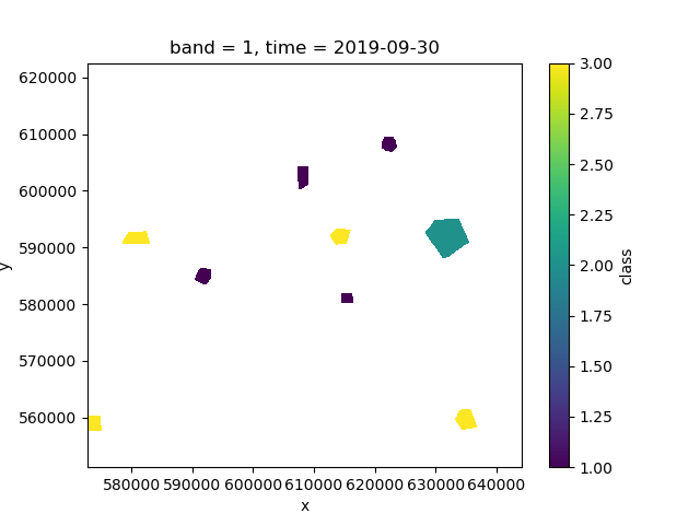
If we investigate labels, we see that it has an associated legend
to match the integer classes:
>>> labels
<xarray.DataArray 'class' (y: 400, x: 400)>
array([[0, 0, 0, ..., 0, 0, 0],
       [0, 0, 0, ..., 0, 0, 0],
       [0, 0, 0, ..., 0, 0, 0],
       ...,
       [0, 0, 0, ..., 0, 0, 0],
       [0, 0, 0, ..., 0, 0, 0],
       [0, 0, 0, ..., 0, 0, 0]])
Coordinates:
    band     int64 1
  * y        (y) float64 6.225e+05 6.223e+05 6.221e+05 ... 5.515e+05 5.513e+05
  * x        (x) float64 5.729e+05 5.73e+05 5.732e+05 ... 6.438e+05 6.44e+05
    time     datetime64[ns] 2019-09-30
Attributes:
    legend:   [(0, None), (1, 'forest'), (2, 'water'), (3, 'nonforest')]
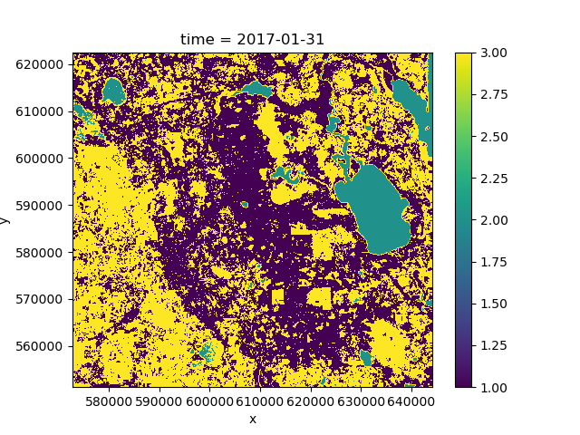
>>> clf = Classifier(RandomForestClassifier(n_estimators=10))
>>> pred = clf.fit(ds, labels).predict(ds)
>>> pred.isel(time=0).plot()
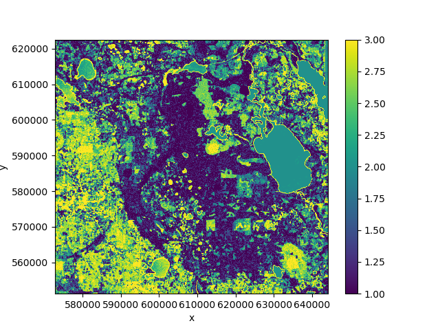
If we plot the mean of the predicted class over time we can see that the predictions change because the forest cover changes over the course of the time period:
>>> pred.mean('time').plot()
7.2. Clustering
Clustering can be done using the same Classifier object because
clustering classes in scikit-learn provide the same interface as classifiers.
Clustering is an unsupervised approach, so the labels argument will be omitted.
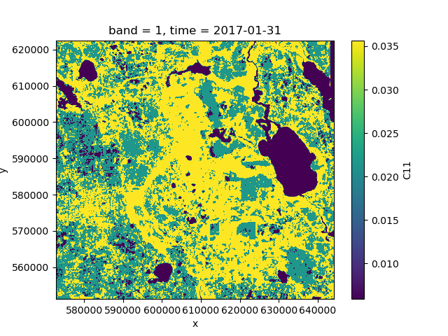
In the following example, we are using nd.classify.class_mean() to replace every
pixel with the mean of its cluster for visualization:
>>> from sklearn.cluster import MiniBatchKMeans
>>> from nd.classify import class_mean
>>> clf = Classifier(MiniBatchKMeans(n_clusters=3))
>>> pred = clf.fit_predict(ds.isel(time=0))
>>> means = class_mean(ds.isel(time=0), pred)
>>> means.C11.plot()
It is advisable to use a clustering algorithm that scales well, such as MiniBatchKMeans.
Alternatively, one can fit the clusterer to a smaller subset of the data by applying a mask.
7.3. Feature and data dimensions
Internally, the entire dataset needs to be converted to a two-dimensional array
to work with most classification algorithm in scikit-learn.
The first dimension (rows) corresponds to independent data points, whereas the second dimension (columns) corresponds to the features (attributes, variables) of that data point.
By default, nd will flatten all dataset dimensions into the rows of the array,
and convert the data variables into the columns of the array.
However, nd.classify.Classifier has an additional keyword argument feature_dims
that controls which dimensions are considered to be features of the data.
Typically, this could be a band dimension, which really isn’t a dimensions but
a set of features (or variables) of the data. It could also be the time dimension,
in which case all time steps are treated as additional information about a point, rather than
separate points in the feature space.
Example:
>>> clf = Classifier(RandomForestClassifier(n_estimators=10),
...                  feature_dims=['time'])
>>> pred = clf.fit(ds, labels).predict(ds)
>>> pred.plot()
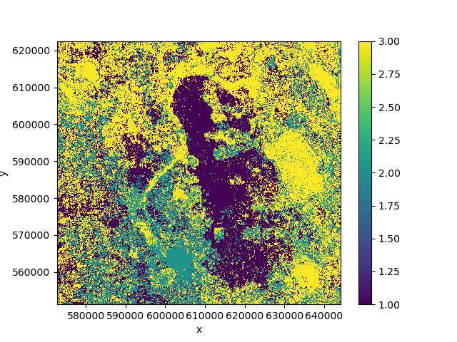
Our prediction output no longer has a time dimension because it was converted into
a feature dimension and used for prediction. In this case the result is not great because
the classes change over time and we thus have noisy training data.
See Also: